Deep learning for audio applications
The rapid advances in deep learning is one of the most interesting technological developments of the past decade. This new technology has many applications in audio processing – ranging from automated assistants that help users making the right choices when producing audio to stem separation, that is separating instrument groups from a complete mix.

Here at HANCE, we focus on the use of deep learning combined with digital signal processing. Our goal is to create solutions based on state-of-the-art academical insight and make them viable in terms of CPU and latency requirements. Some of the use cases of our technology are:
- Separation of complete mixes into stems (instrument groups)
- Dialogue extraction from background noise
- Reduction of unwanted reverberation
- Spectrogram inpainting – fill holes in time/frequency
- Bandwidth expansion – recover lost content in specific frequency ranges
Source separation
Stem and vocal separation has been a popular topic in academic research during recent years. Stem separation, dialogue extraction and reverb reduction are closely related problems that can be tackled with the same neural network structure, but with different training sets. We will use the term source separation to describe the general problem. Some source separation methods that deliver state-of-the-art results are:
- Open-Unmix (spectrogram processing)
- Demucs (waveform processing)
- MMDenseLSTM (spectrogram processing)
- Spleeter (spectrogram processing)
While these methods provide astonishing results, they are not well suited for real-time processing as they introduce too much latency and have demanding memory and CPU (or GPU) requirements. We will focus on spectrogram-based separation as it is generally less computationally expensive than waveform-based separation and the U-Net structure has proven very effective.
Brief overview of current methods
Spectrogram based methods
Spectrogram-based methods for source separation typically estimate a separation mask that is multiplied pointwise with the input magnitude spectrogram to form the separated output magnitude spectrogram. For simplicity, the output audio is commonly reconstructed using the phase information from the input spectrogram. By processing magnitude spectrograms this way, we can easily adopt network topologies that have been implemented for image processing by treating the magnitude spectrogram as a gray-scale image.


Convolutional neural networks
Convolutional Neural Networks (CNNs) have their origin in image classification and processing. The basic idea is to apply a set of strided 2D convolutions with trainable weights, that reduce the resolution while increasing the number of channels. An activation function is applied to the output, such as the Rectified Linear Unit (ReLU) that simply sets all negative values to zero. The procedure is repeated to form layers with decreasing resolution and an increasing channel count.
In network for classification, there is typically a fully connected layer at the end. For audio processing tasks, however, we are more interested in reconstructing a separation mask as described earlier. We can achieve this by adding an upsampling stack of layers that increases the resolution in each step until we have the original resolution. This is achieved by reversing the operations in the downsampling layers. The resolution is increased and a set of 2D convolutions with trainable weights are applied – a process usually referred to as transposed convolution (or sometimes incorrectly as deconvolution). Similar to the downsampling layers, an activation function is applied after the transposed convolution. The resulting topology is similar to so called auto-encoders, but with a spectral separation mask as desired output.

U-Net
The U-Net is an extension of the CNN auto-encoder that adds so called skip connections between layers at the same level in the encoding and decoding stacks. It was first proposed for medical image segmentation in the article U-Net: Convolutional networks for biomedical image segmentation and was used for audio source separation in the article Singing Voice Separation with Deep U-Net Convolutional Networks.

The skip connections ensure that important locational information is not lost in the encoding and decoding stacks.
Latency hurdles
Due to the image processing legacy of the U-Net topology, the implementations have not been well suited for real-time processing due to the huge latency introduced. Audio is divided into long time chunks and the magnitude spectrogram is calculated before the actual separation can take place. One example of this approach is the pre-trained Spleeter models that have been integrated into several commercial applications, including Acon Digital Acoustica, iZotope RX8 and Steinberg SpectraLayers. The original Spleeter implementation processes chunks of around 11 seconds of audio which is of course way more that acceptable for real-time processing.
Pre-processing in a background thread is used to allow remixing during playback in the most advanced commercial offerings, but this is of course not an option in applications such as video conferencing or even when implementing audio plug-ins in one of the common formats, such as VST, Audio Units or AAX.
HANCE Audio Engine
Real-time processing requires a fundamentally new approach. The HANCE Audio Engine (HAE) is a model inference library that is very light-weight and optimized for time-continuous data. It interprets the magnitude spectrogram as a stream of time frames. These time frames are pushed to the audio engine which delivers output time frames with the shortest possible latency that the model allows.
Each layer in the model only holds input data as long as necessary. I.e., a convolution layer will only hold as much history as required to compute a single output frame and will forward data as soon as possible. This way, both latency and memory requirements are minimal.
Adapting the model
So, how long is the latency we can expect with the stream-based approach in the HANCE Audio Engine? The Spleeter implementation uses six layers, each with 5 x 5 convolution kernels and a downsampling factor of two. The latency increases exponentially in the downsampling layers, and we need to feed the neural network 254 frames before we receive the first frame at the output. With an FFT size of 4 096 samples and a hop size of 1 024 samples, the latency is a whopping 1 024 x 254 = 260 096 samples. The model is trained on audio sampled at a 44.1 kHz rate, so the latency corresponds to 5.90 seconds – not anywhere near real-time.
We found that it is possible to reduce this latency substantially. One of the key elements is to use time causal 2D convolution that only depends on previous input. This is of course especially important for the low-resolution layers where the impact on the total latency is highest. The separation quality does improve dramatically for the first few frames of look-ahead, but the increase in separation quality drops quickly as further look-ahead frames are added.
Training and HAE files
Currently, training is done with the Keras and TensorFlow frameworks. The network topology along with kernel weights and other trained variables can be exported to a compact HANCE file. These files contain all the information necessary for the model inference and can be loaded in our cross-platform HANCE inference engine. This makes it very easy to implement audio processing based on deep learning for a wide variety of tasks.
Results
We have trained several HAE models so far with an emphasis on dialogue enhancement. Our dialogue noise reduction model is trained on a large set of dialogue recordings made under ideal conditions and recordings of common noise sources. The audio was recorded at 48 kHz and the model uses a block size of 2 048 samples and a hop size of 512 samples.
We tuned the parameters towards a latency that is acceptable for a plug-in intended for post-production work. Especially for impulsive noises, the separation improves notably when allowing some latency, and latencies up to around 100 milliseconds are acceptable for use in post-production.
The resulting model introduces seven frames latency, corresponding to 3 584 samples. The short time Fourier transform (STFT) will add additional latency depending on the input block size. With the ideal case of having an input block size of 2 048, the STFT will introduce a latency equal to the hop size. The total latency sums up to 4 096 samples in this case which corresponds to 85 milliseconds.
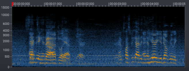
The results of the network topology described in this article on a noisy interview. Please use the switch in the player to toggle the processing on and off.
Despite the amazing noise reduction capabilities of the model, there are still noticeable chirp like artifacts introduced by the algorithm. By adding custom layers and tuning the loss function, we were able to reduce the artifacts significantly without adding additional latency, and only an insignificant increase in the CPU usage. We also extended the training set.
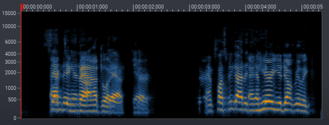
The results of an improved network topology that reduces chirp like artifacts on the same noisy interview as above. Please use the switch in the player to toggle the processing on and off.